
Conformer: Combining CNNs and Transformers for Speech Recognition
Published:
Conformer
Conformer is a model architecture popularly used in automatic speech recognition (ASR), which combines the strengths of CNN and Transformer by deeply integrating these two structures. To have a deep understanding of it, we should not only remember its components, but also understand why it’s designed in that way.
Where Conformer Fits in an ASR Pipeline
A modern ASR system typically follows an encoder + CTC / transducer / attention-decoder structure. The encoder consumes audio features (e.g. log-mel spectrograms) and transforms them into high-level, contextualized acoustic representations that summarize what was said at each time step. The CTC head, transducer, or attention decoder then maps these representations into text tokens — CTC emits a per-frame token distribution under a conditional-independence assumption (frames are independent given the encoder output), while transducers and attention decoders additionally condition on previously emitted tokens when generating the next one.
Conformer sits on the encoder side of this pipeline. It does not produce text directly; instead, it produces the rich acoustic features that the downstream head decodes into a transcript.
Attention vs. Convolution
Before diving into the detailed architecture of Conformer, it’s worth understanding the contrast between attention and convolution — the choice to fuse the two is precisely what distinguishes Conformer from a vanilla Transformer.
Attention
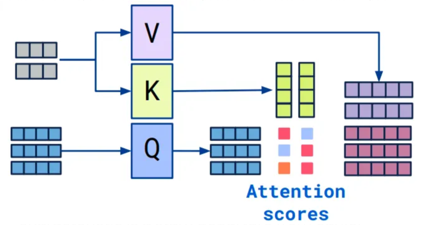
The figure above illustrates the attention mechanism. There are two streams of inputs: the blue tensors act as “finders” looking for information, and the grey tensors act as “candidates” that may carry useful information. The operation proceeds in three steps.
1. Project. The blue inputs are linearly projected into query tensors. The grey inputs are projected by two separate linear layers into key and value tensors.
2. Score. For each query, a dot product is computed against every key, yielding a raw relevance score for each query–key pair. Intuitively, the query is a “missing-person sketch” and each key is a “candidate photo”; the dot product measures similarity. The scores are then scaled by 1/√d_k and passed through a softmax to produce attention weights that sum to 1.
3. Aggregate. The values are combined as a weighted sum using those attention weights, producing the output for each query.
In an audio encoder, the blue and grey inputs are the same tensor — this is called self-attention. Each tensor carries information from one time frame, and self-attention lets every frame gather information from every other frame (including itself). Because any frame can directly attend to any other frame in a single layer, attention captures global, long-range context uniformly, regardless of where the frames sit in the sequence.
Convolution
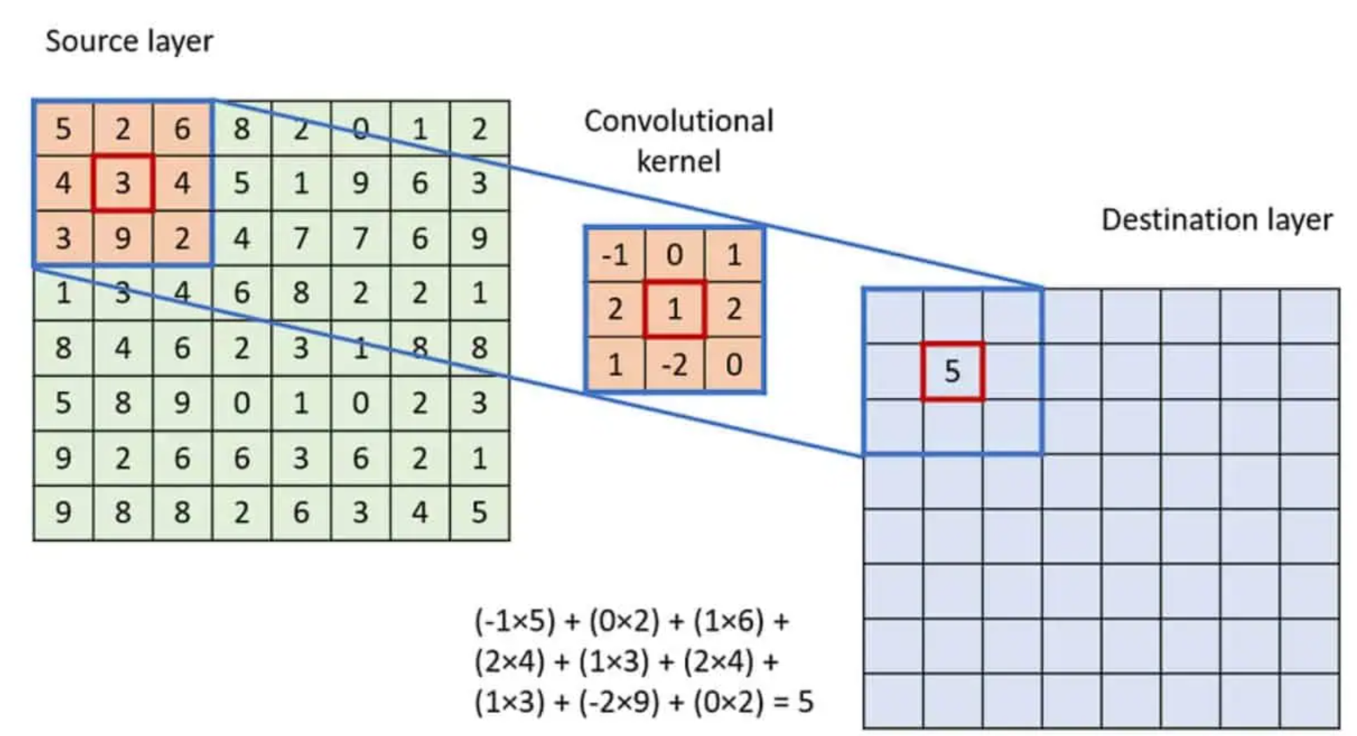
Convolution applies a learned filter (kernel) that slides across the input and computes a weighted sum over a fixed window around each position. Because that window is small — typically just a handful of frames — a single convolution layer only sees a narrow local neighborhood. Stacking convolutional layers grows the receptive field, but only gradually.
The takeaway: convolution excels at local patterns but struggles with long-range dependencies — the exact complement of attention. Conformer’s design fuses the two so that each block can model local and global structure together.
Conformer Block Overview
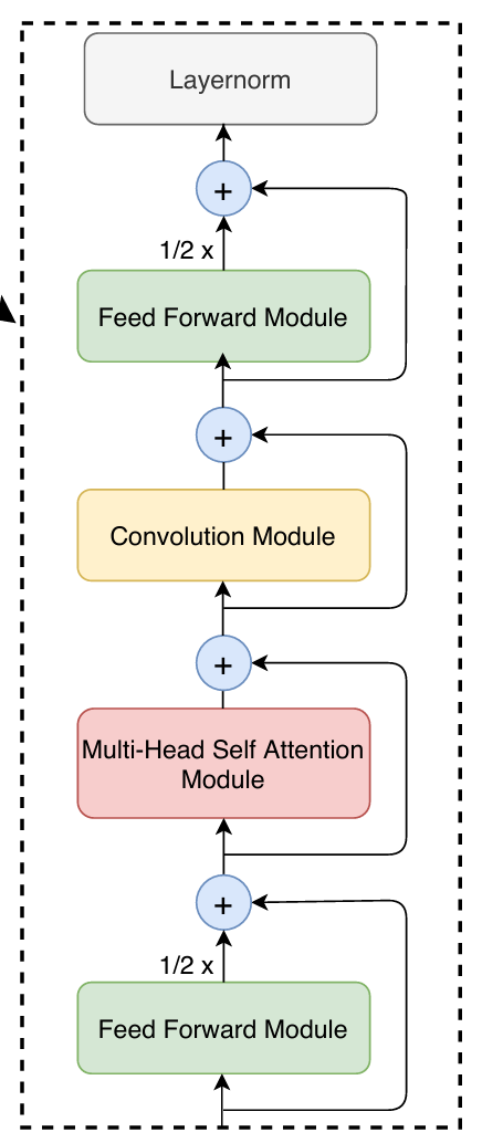
Now, let’s look at the detailed architecture of Conformer. The core of the Conformer architecture is the conformer block, which essentially has 5 components: Feed Forward Module (FFN) → Multi-Head Self Attention Module (MHSA) → Convolution Module → Feed Forward Module → Layernorm. These chain of operations can be formulated as:
\[\begin{aligned} x_{2} &= x_{1} + 0.5*FFN_{1}(x_{1})\\ x_{3} &= x_{2} + MHSA(x_{2})\\ x_{4} &= x_{3} + Conv(x_{3})\\ x_{5} &= x_{4} + 0.5*FFN_{2}(x_{4})\\ x_{6} &= Layernorm(x_{5}) \end{aligned}\]At a glance: a Conformer block sandwiches an MHSA → Conv pair between two half-weighted FFNs — the Macaron-style structure borrowed from Lu et al. (2019). The MHSA, inherited from the Transformer, captures global context, while the Conv module captures local patterns; this complementary pairing is what lets Conformer outperform a vanilla Transformer on tasks like ASR.
In the following, I will dive into several components where I think the design choices deserve closer attention.
Convolution Module
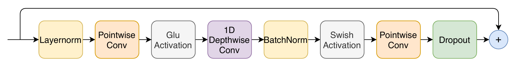
The precise sequence of the Convolution Module is: LayerNorm → Pointwise Conv(d_model, 2·d_model) → GLU → Depthwise Conv(d_model, d_model, kernel=31) → BatchNorm → Swish → Pointwise Conv(d_model, d_model) → Dropout, with a residual connection around the entire module.
The convolution module employs a depthwise separable convolution, preceded by a pointwise convolution that expands the channel dimension to 2× d_model for GLU activation. GLU splits the expanded tensor into two halves and computes σ(gate)⊙value, providing learnable channel-wise gating.
FFN
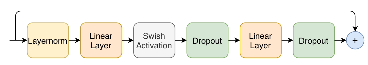
The precise sequence of the FFN is: LayerNorm → Linear(d_model, 4·d_model) → Swish → Dropout → Linear(4·d_model, d_model) → Dropout, with a residual connection around the entire module.
The noteworthy part is that it takes an inverted bottleneck structure, where it provides a larger representational space for the nonlinear activation to operate in.
Inference Flow
Understanding how the data went through each operation in a model is important to have a more concrete understanding of the model, rather than just have an intuitive but blurry understanding. In the following, I would take you experience how the data shape changes when using Conformer in real ASR applications.
1. Raw Audio Input
Everything starts with a raw waveform. In a typical ASR pipeline, you receive audio sampled at 16,000 Hz.
Input waveform: (B, T_samples)
  e.g. (4, 64000)  →  4 utterances, each 4 seconds long
2. Feature Extraction — Log-Mel Spectrogram
The raw waveform is first transformed via a Short-Time Fourier Transform (STFT) — using, for example, a 25ms window and 10ms hop — to produce a spectrogram, which is then mapped through a mel filterbank and log-compressed to yield the log-mel spectrogram.
- Frames =
T_samples / hop_length≈64000 / 160= 400 frames - Mel bins = 80 (standard in ESPnet / WeNet setups)
After feature extraction: (B, T, F)
  e.g. (4, 400, 80)
3. SpecAugment (Training Only)
Time and frequency masks are applied to the feature tensor. The shape does not change — values are just zeroed out in certain bands.
After SpecAugment: (4, 400, 80) ← same shape
4. Subsampling (Conv2D Subsampler)
To reduce the sequence length (which is expensive for attention), a Conv2D subsampling module is applied — typically with stride 2 twice, giving a 4× reduction. This shrinks the time dimension to make attention more tractable. Besides, the frequency dimension is reduced during this subsampling as well (e.g. 400→100 frames and 80→20 mel bins).
The feature map is first treated as a 2D image (T, F), convolved, then reshaped into a 1D sequence projected to the model dimension d_model (e.g. 256).
Before subsampling: (4, 400, 80)
Add channel dimension: (4, 1, 400, 80)
Conv2d subsampling: (4, 256, 100, 20)   ← more channels, fewer frequency bins and time frames
Reshape: (4, 256, 100, 20) → (4, 100, 256×20) → (4, 100, 5120)
Linear projection: (4, 100, 256)   ← T//4, d_model
This is why ASR Conformers are tractable — attention runs over 100 frames, not 400.
5. Positional Encoding
A sinusoidal (or relative) positional encoding of shape (1, T', d_model) is added to the sequence. Shape is unchanged.
After positional encoding: (4, 100, 256)
6. Conformer Block (×N)
Each Conformer block is composed of four sub-modules in sequence. Let’s trace shape through one block:
6a. Feed-Forward Module (first half, scale ½)
A two-layer FFN with expansion factor 4:
Input          : (4, 100, 256)
After Linear_1 : (4, 100, 1024)   ← expand
After Swish    : (4, 100, 1024)
After Dropout  : (4, 100, 1024)
After Linear_2 : (4, 100, 256)    ← project back
6b. Multi-Head Self-Attention Module
With num_heads = 4 and d_model = 256, each head has d_k = 64:
Input          : (4, 100, 256)
Q, K, V        : each (4, 4, 100, 64)   ← (B, heads, T, d_k)
Attention scores: (4, 4, 100, 100)
After softmax  : (4, 4, 100, 100)
Context        : (4, 4, 100, 64)
After reshape  : (4, 100, 256)
After out proj : (4, 100, 256)
6c. Convolution Module
A depthwise convolution with kernel size 31 operates along the time axis:
Input               : (4, 100, 256)
After pointwise_1   : (4, 100, 512)   ← GLU doubles channels
After GLU           : (4, 100, 256)   ← halves back
After depthwise conv: (4, 100, 256)   ← kernel=31, same padding
After BatchNorm     : (4, 100, 256)
After Swish         : (4, 100, 256)
After pointwise_2   : (4, 100, 256)
6d. Feed-Forward Module (second half, scale ½)
Same as 6a. Output shape stays (4, 100, 256).
After all N=12 Conformer blocks (typical for medium-size models), the shape is still:
After N Conformer blocks: (4, 100, 256)
7. CTC / Attention Decoder Head
Depending on the decoding strategy:
CTC Head — a linear projection over the vocabulary (e.g. 5000 BPE tokens):
After Linear  : (4, 100, 5000)
After LogSoftmax: (4, 100, 5000)   ← per-frame token log-probs
Attention Decoder — an autoregressive Transformer decoder cross-attending to the encoder output, producing one token at a time:
Encoder output : (4, 100, 256)
Decoder input  : (4, L_text, 256)   ← L_text = target length
Cross-attention: keys/values from encoder, queries from decoder
Final output   : (4, L_text, 5000)
Summary Table
| Stage | Shape |
|---|---|
| Raw waveform | (B, T_samples) |
| Log-Mel features | (B, T, 80) |
| After subsampling | (B, T/4, 256) |
| After each Conformer block | (B, T/4, 256) |
| CTC output | (B, T/4, vocab_size) |
| Decoder output | (B, L_text, vocab_size) |
The key insight is that the sequence length shrinks early (at the subsampler) — this is what makes the self-attention computationally feasible and then stays constant all the way through the Conformer stack. The model dimension d_model is similarly fixed throughout, acting as a consistent “information highway” between modules.
Leave a Comment