Paper Reading: Overcoming Catastrophic Forgetting in Neural Network

Background

One way to address catastrophic forgetting is to introduce regularization when learning new tasks. The idea is straightforward: continue learning the new task while applying regularization to prevent the model from forgetting what it learned from previous tasks. The tricky part is figuring out how to apply this regularization effectively. The paper “Overcoming Catastrophic Forgetting in Neural Networks” proposes a method called Elastic Weight Consolidation (EWC), which offers one such solution.

Fisher Information

From my point of view, the core idea of Elastic Weight Consolidation (EWC) is grounded in Fisher Information. If you develop a solid understanding of Fisher Information, you’ve essentially grasped 90% of the paper. However, the concept can be quite abstract, especially for those without a strong background in statistics. Personally, despite having a basic understanding of probability, it took me over 10 hours to truly grasp the foundational idea of Fisher Information.

In the following, I’ll walk you through Fisher Information from a beginner’s point of view. Some terminology may be simplified and not strictly rigorous, but the explanation should be sufficient to help you understand the core intuition behind the paper.

Problem to Solve

Let’s begin with the problem context. Imagine we have a set of data points that are assumed to come from a known family of probability distributions. Our goal is to estimate some unknown parameters of this distribution using the observed data.

For example, suppose the data points are drawn from a Gaussian distribution, but we don’t know the mean or variance. How precise can our estimation of the parameters can be, given the data? Fisher Information provides a way to quantify that.

But before we define Fisher Information, let’s revisit a fundamental concept: likelihood.

Likelihood

Most of us are familiar with probability. Given a distribution parameterized by some variable $\theta$, the probability tells us how likely a specific data point $x$ is under that distribution. If the data point is continuous, we can represent its probability using a probability density function, denoted as $p_{\theta}(x)$. In this case, $x$ is the variable, and $\theta$ is fixed.

In contrast, likelihood flips the perspective. Given an observed data point $x$, likelihood asks: How does the probability of observing this data change as the parameter $\theta$ varies? There are two things noteworthy here:

• Likelihood is a function of the parameter $\theta$, with the data $x$ fixed.
• It is usually proportional to the probability density evaluated at $x$ for a given $\theta$.

Mathematically, we write the likelihood as: $L(\theta\vert x) = p_{\theta}(x)$. Even though it looks the same as the PDF, the interpretation is different: here, we treat $x$ as fixed and view $L$ as a function of $\theta$. With a basic understanding of likelihood in place, let’s now return to the concept of Fisher Information.

Now to Fisher Information

Mathematically, Fisher Information is denoted as:

This formula can be broken down into two main parts:

1. The integrand: $(\frac{d}{d\theta}log(p(x \vert \theta))^2$, which is the square of the derivative of the log-likelihood with respect to the parameter $\theta$.
2. The integration: Taking the expectation over all possible values of $x$, weighted by their likelihood under the current parameter $\theta$.

The integration is straight forward while the integrand is complicate. Let’s unpack the intuition behind the integrand step-by-step.

• First, note that the log is used for mathematical convenience—it turns products into sums and simplifies derivatives. Since it’s a monotonic function, it doesn’t fundamentally change where the likelihood peaks or how sensitive it is to $\theta$. So for intuition, we can temporarily set aside the log and focus on the likelihood itself.
• Next, the derivative of the likelihood (or log-likelihood) with respect to $\theta$ tells us how sensitive the probability of observing data point $x$ is to changes in the parameter. In other words, it measures how much the likelihood shifts when $\theta$ is nudged.
• Then, the square of the derivative simply removes the sign and emphasizes the magnitude—ensuring that both increases and decreases in likelihood contribute positively to the overall measure.

Putting this together:

If the derivative is close to zero, it means that small changes in $\theta$ don’t affect the likelihood much. This suggests that $x$ doesn’t contain much information about $\theta$ at that value because nearby values are almost the same likely to generate the same $x$, and thus, we can’t estimate $\theta$ very precisely based on $x$—the Fisher Information is low. Conversely, if the derivative is large, the likelihood is very sensitive to $\theta$, meaning $x$ can locate $\theta$ well—the Fisher Information is high.

Now, I think you’ve got a basic understanding of why Fisher Information can manifest the sensitivity of data $x$ to parameter $\theta$.

Back to EWC

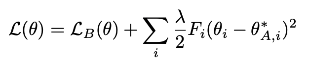
Let’s return to EWC. At its core, Elastic Weight Consolidation (EWC) is based on the above loss function, which consists of two components. The first is the standard loss for task B (the new task), and the second is a regularization term. In this term, $F$ denotes the Fisher Information Matrix, $\theta$ represents the current weights being optimized, and $\theta_A^*$ refers to the weights previously learned for task A (the old task). $\lambda$ is a hyperparameter that controls the strength of the regularization, and $i$ indexes the model parameters.

In other words, weights associated with higher Fisher Information—meaning small changes in them would significantly affect the likelihood—are considered more critical for preserving performance on previous tasks. EWC penalizes changes to these important weights more heavily, thereby preventing the model from “forgetting” them when learning new tasks. This is how Fisher Information is used to guide the regularization in EWC and mitigate catastrophic forgetting.

The paper also provides a theoretical justification for the form of the loss function, even though the intuition is quite clear. For a more formal understanding, you can refer to Equations (1) and (2) in the paper, which are relatively straightforward to derive.

In the experimental section, the authors evaluate EWC on both a classic benchmark—Permuted MNIST—and reinforcement learning tasks. The results show that EWC outperforms vanilla SGD and L2 regularization in terms of maintaining performance across tasks. We won’t go into the experimental details here.

Conclusion

“Overcoming Catastrophic Forgetting in Neural Networks” is a classic paper in the field of continual learning. It presents a clear narrative, combining intuitive ideas with solid mathematical foundations, and supports them with well-designed experiments that demonstrate the method’s effectiveness. While fully grasping every detail may require a strong background in statistics or some additional reading, the paper is absolutely worth revisiting multiple times to understand the reasoning behind its approach.